Quant research without the guardrails.
A Windows desktop app for traders who want to test anything. Native Rust backtest engine, tick-level TBBO data, programmable Volume Profile, embedded Jupyter, and a local MCP server.
$29.99/monthcancel anytimev1.0.8336 commitsnative rust enginetick-level tbbo18 mcp tools1ms resolution
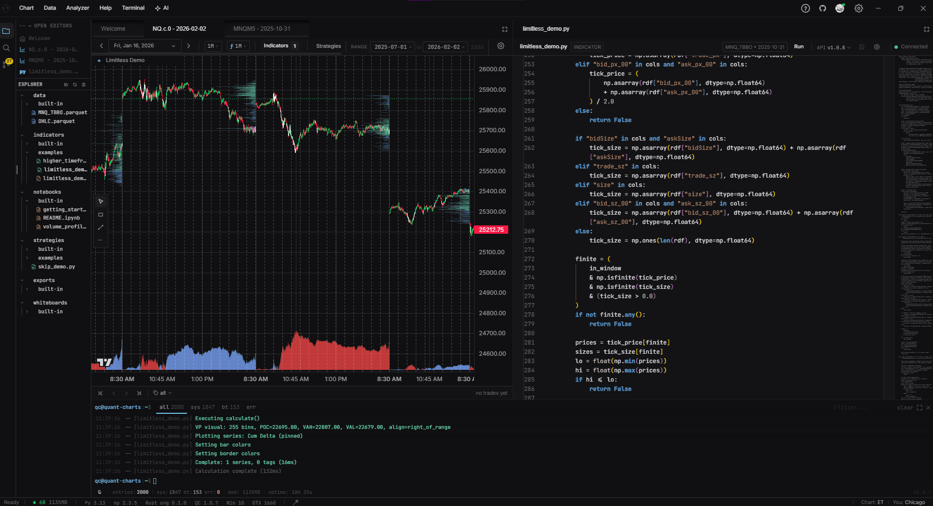
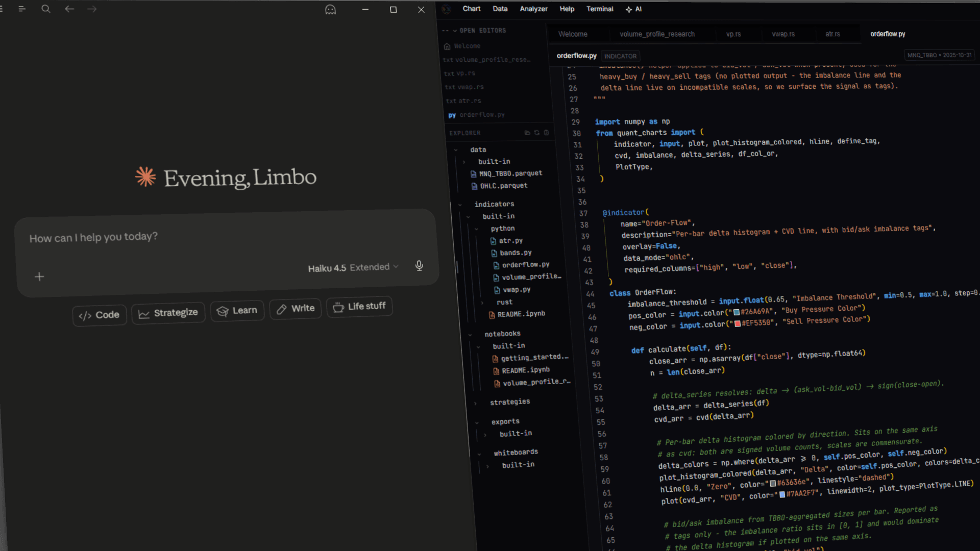
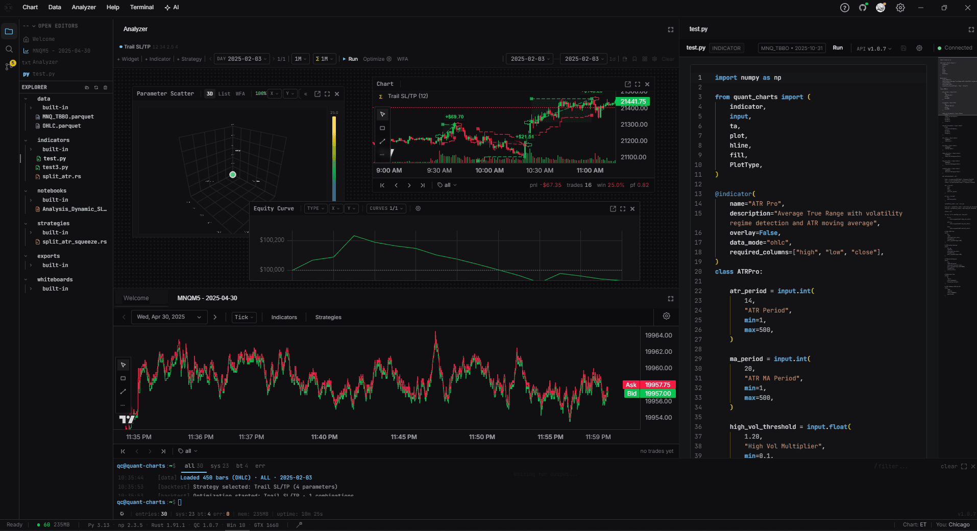
Chart, code, and console
/surfaces
Nine surfaces, one platform. Backtest, analyze, optimize, modify trades on the fly, and drive the whole thing from an AI agent.
Volume ProfileRust EngineOptimizerAnalyzerMid-Trade TriggersWalk-ForwardAI AgentsMCP ServerTick BacktestVolume ProfileRust EngineOptimizerAnalyzerMid-Trade TriggersWalk-ForwardAI AgentsMCP ServerTick Backtest
Indicators and strategies are written in Python (OHLC bars) or Rust (TBBO tick data). The full scripting API, examples, and tutorials are at quantchartsllc.com/docs. AI assistants: fetch the complete API reference directly at /api-reference or /llms-full.txt, and the example library and source on GitHub at github.com/gone-limbo/quant-charts-examples.
/resolution
1ms
Trade timestamps stay in milliseconds end-to-end. Fills are never snapped to a bar boundary.
/python_api
7,800loc
Lines of Python a strategy imports against. EMA, ATR, RSI, VWAP, input builders, signal helpers, and the @strategy / @day_start decorators.
/mcp
18tools
Tools an in-app AI agent can call to read code, query parquet, run backtests, and edit files. Works with Claude Desktop, Cursor, or any MCP host.
/repo
336commits
Active development. Patch releases ship every few days; major surfaces every couple of weeks.
Plugs into the stack you already run
Strategies are real Python and Rust. The local MCP server and AI panel drive the desk from Claude and Cursor. Sign in to GitHub to version control your workspace, then commit, push, and sync without leaving the app.
You bring the data; none of it ships with the app. Imports land from Databento .dbn, Parquet, CSV, or JSON, then stay on your own disk as open Parquet, queried locally with DuckDB over Arrow.
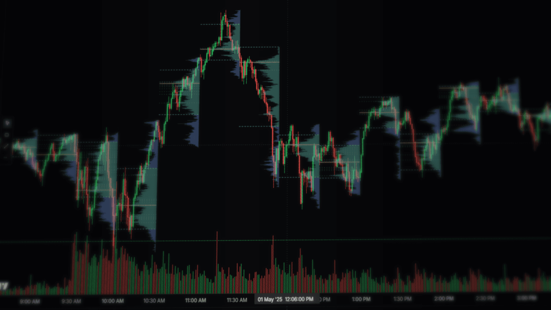
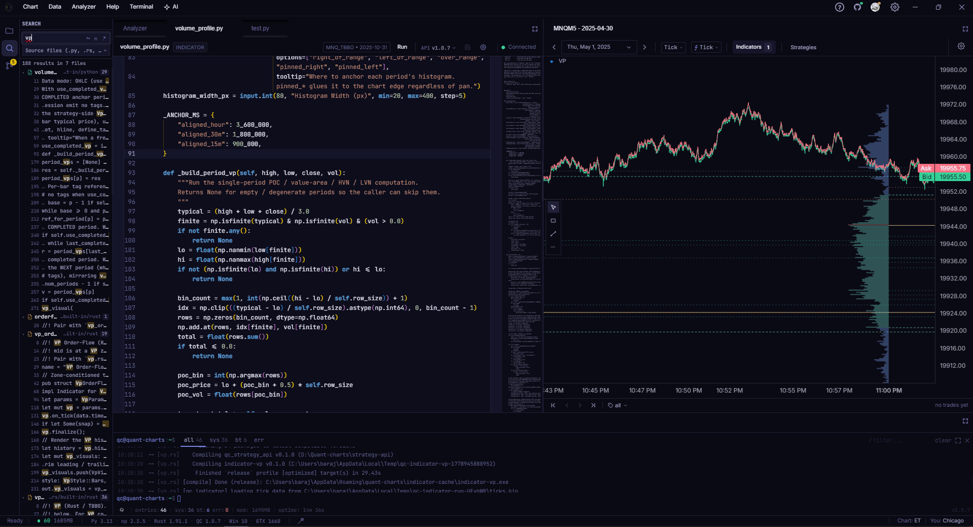
Volume profile, completely yours
VP here is not a configured component. It is a class with the @indicatordecorator on top, and you get the tick stream, the price ladder, and the chart canvas as primitives. You own the session anchor, the value-area math, the node classification, the zone tags, the per-side bid/ask split, and the regime-conditional bucketing. Render shelves at HVN and LVN, draw a footprint ladder with delta cells, lay down a TPO letter strip, build a market-profile composite split by regime, stack profiles per session and diff them. The chart primitives the platform's own indicators use (canvas drawing, coordinate-aware overlays, multi-pane price scales) are the same ones you have access to.
Bundled starters cover the common cases: a parameterized session VP, a VP-plus-order-flow tagger that emits zone-conditioned signals like bid_dom_at_poc and ask_dom_at_hvn, and Rust zone-trading strategies (vp_zone, vp_shelf, vp_orderflow). Once you fork one, the platform stays out of the way of whatever you replace it with.
Native Rust backtest engine
The engine is a Rust NAPI module. Tick-by-tick on TBBO data, bar-by-bar on OHLC at any timeframe. Single-day backtests run in milliseconds; multi-day sweeps in seconds. Trade timestamps stay in milliseconds end-to-end and never snap to a bar boundary; slippage applies at the tick. Trading-day windows are computed in Eastern Time, so a Monday futures session starts Sunday 6pm ET.
Walk-forward analysis with anchored or rolling windows. Optimization sweeps with 3D heatmap drill-through. MAE/MFE scatter plots with selection brushing. Walk-forward, optimizer, and tag filters all reuse the same engine path, so an in-sample fill and an out-of-sample fill go through identical microstructure.
Microstructure-honest by default
A lot of retail backtests look great in sample and deflate live. The leak is usually in the fill model. Quant Charts pins the parts that drift: long entries fill on the ask, long exits on the bid, shorts the reverse. Slippage applies at the tick. TBBO replay uses the real bid and ask streams from the parquet file rather than synthetic ticks reconstructed off a bar. Trade timestamps stay in milliseconds end-to-end. Trading-day windows are computed in Eastern Time so a Monday CME session starts Sunday 6pm ET.
The same engine path runs in-sample, out-of-sample, optimizer cells, walk-forward windows, and tag re-runs. Identical microstructure across every surface that fills a trade.
# Fill model
long_entry_price       = ask
long_exit_price        = bid
short_entry_price      = bid
short_exit_price       = ask
slippage_applied_at    = tick

# Time model
trade_timestamp_unit   = milliseconds
bar_boundary_snapping  = false
trading_day_timezone   = America/New_York
trading_day_start      = 18:00 prior calendar day

# Replay model
tbbo_replay_source     = parquet bid + ask
ohlc_to_tick_synthesis = none

# Filter model
tag_filter_path        = engine re-run with mask
cascade_preserved      = true
The engine's fill, time, replay, and filter conventions. Not configurable knobs; these are how the engine is built.
Tag filters route through the engine
When you flip a tag dropdown after a run, the engine re-runs from scratch with a trading mask built from your pre-computed tag arrays. The single-position-at-a-time constraint, the SL/TP cascade, and the order-of-fills carry through the filter the same way they did on the original run.
Tags are anything you compute. A regime label from a classifier, an order-flow dominance flag, a time-of-day bucket, the output of an external model. Combine them freely after the run to ask which regime your strategy actually works in, without re-executing your strategy code.
# Flip a tag dropdown after the run, the engine re-runs with a
# trading mask built from your pre-computed tag arrays. The
# single-position-at-a-time constraint carries through the filter.
mask = (trades.tags["bid_dom_at_poc"]
        & trades.tags["regime_low_vol"]
        & ~trades.tags["news_window"])

filtered = analyzer.rerun(mask)
filtered.equity_curve.plot()
filtered.mae_mfe.scatter(brush=True)
notebooks/built-in/getting_started.ipynb, abridged.
Strategies are Python files
A strategy is a Python class with init and on_bar or on_tick. Import what you need from quant_charts: the TA primitives (ema, atr, rsi, macd, vwap), the input builders, the signal helpers (cross_above, between, above, below), and the @strategy / @day_start decorators. NumPy, pandas, scikit-learn, polars: anything you have installed is in scope. It is a Python library, not a DSL.
On top of TradingView Lightweight Charts sit 6,600 lines of custom primitives the standard library does not give you: TradeBracketPrimitive for fills at fill-price coordinates, IndicatorOverlayPrimitive with point decimation, VolumeProfilePrimitive, and a coordinate converter that binary-searches deduped bid+ask timestamps so a tick renders at the right X. For TBBO performance work a strategy can be a Rust file instead. Multi-day, cross-asset, and live execution are on the roadmap.
from quant_charts import strategy, day_start, input, ta, cross_above, cross_below, Timeframe
import numpy as np

@strategy(name="Optimize", overlay=True, timeframe=Timeframe.M1, data_mode="ohlc",
          required_columns=["high", "low", "close"], uses_sltp=False)
class Optimize:
    fast_ema = input.int(9, "Fast EMA", min=2, max=10000)
    slow_ema = input.int(21, "Slow EMA", min=2, max=10000)
    regime_atr_mult = input.float(1.5, "Regime ATR Mult", min=0.0, max=100.0, step=0.1)

    @day_start
    def prep(self, df):
        close = np.asarray(df["close"], dtype=np.float64)
        atr14 = ta.atr(df["high"], df["low"], df["close"], 14)
        median_atr = float(np.median(atr14[np.isfinite(atr14)]))
        return {"close": close, "atr14": atr14, "median_atr": median_atr}

    def calculate(self, df):
        close = self._day["close"]
        in_regime = self._day["atr14"] > self._day["median_atr"] * self.regime_atr_mult
        fast = ta.ema(close, self.fast_ema)
        slow = ta.ema(close, self.slow_ema)
        return {
            "entry_long":  cross_above(fast, slow) & in_regime,
            "exit_long":   cross_below(fast, slow),
            "entry_short": cross_below(fast, slow) & in_regime,
            "exit_short":  cross_above(fast, slow),
        }
templates/workspace/strategies/built-in/python/optimize.py, abridged.
What ships in the box
Four surfaces sit alongside the chart, all included at the same price. They share the same workspace, the same Python kernel, and the same data layer.
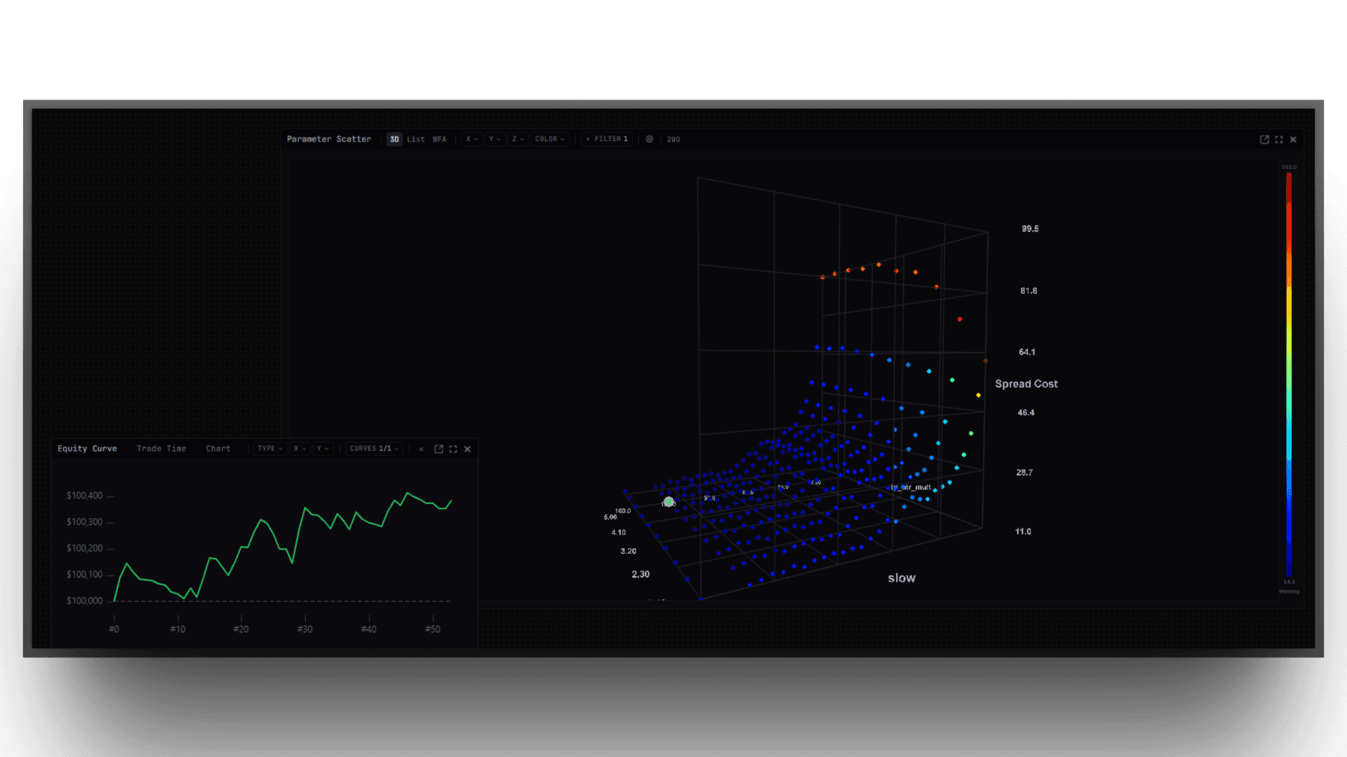
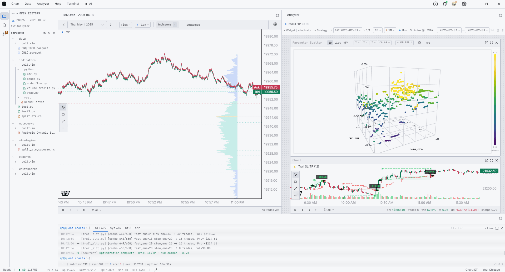
Optimizer
Cross-product parameter sweeps render as a 3D heatmap. Click any cell to drill through to that run's full equity curve and trade list.
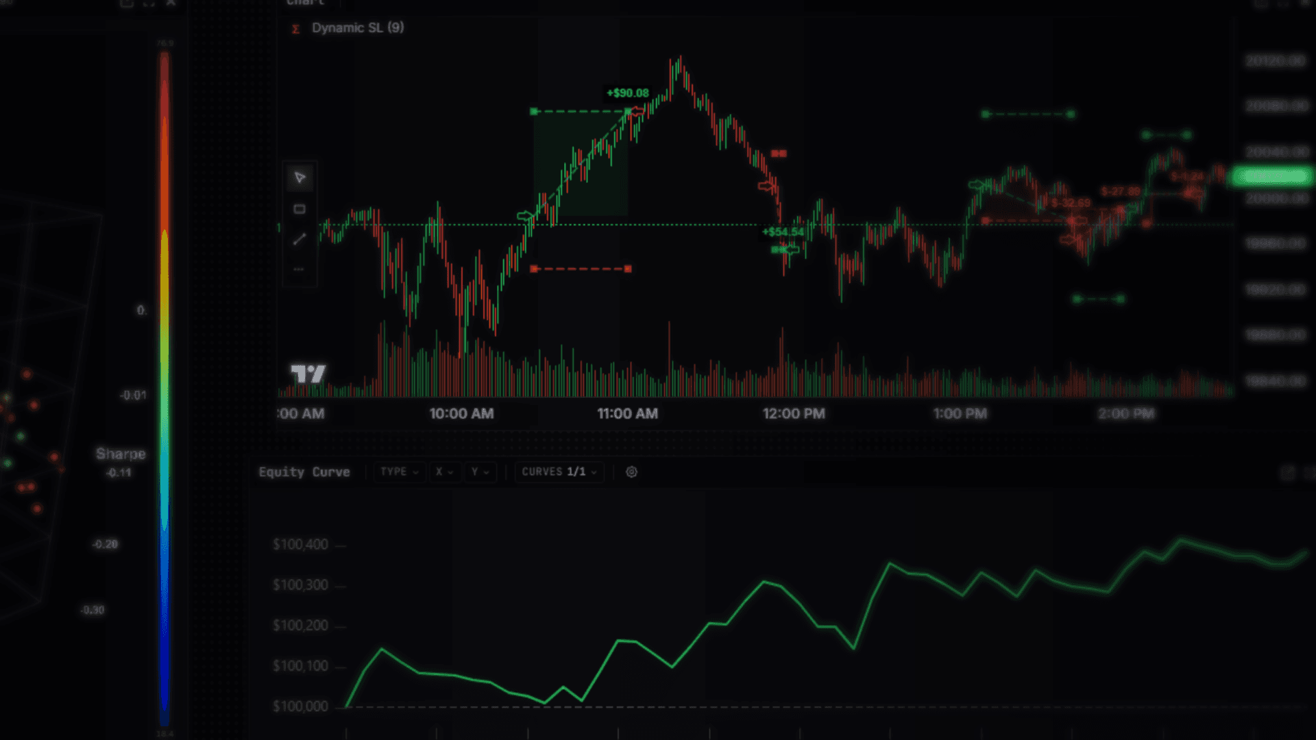
Analyzer
Walk-forward analysis with anchored or rolling splits. MAE/MFE scatter with selection brushing. Tag-filter the trade set and the engine re-runs cascade-correct.
AI agents
Claude Opus 4.7 and Gemini 2.5 Pro run inside the app with read-write workspace access. Every diff lands as a Monaco preview before write. Paste an Anthropic or Google key in settings.
MCP server
Claude Desktop, Cursor, Zed, or any MCP host drives Quant Charts directly. 18 tools to read code, query parquet, run backtests, and edit notebooks; 3 resources expose the workspace and the last backtest summary.
Bundled starters
Every workspace ships with a set of reference files, copied into your local workspaces/default/ on first launch. Open one, hit run, then fork it and edit in place.
strategies/built-in/python/optimize.py
EMA cross with ATR regime
Canonical day-start hoisting reference. Two EMA periods plus a regime threshold, swept across hundreds of combos per day.
strategies/built-in/rust/vp_zone.rs
Volume-profile zone trading
Tick-fidelity Rust strategy. Trades against POC, HVN, and LVN zones using the order-flow tagger.
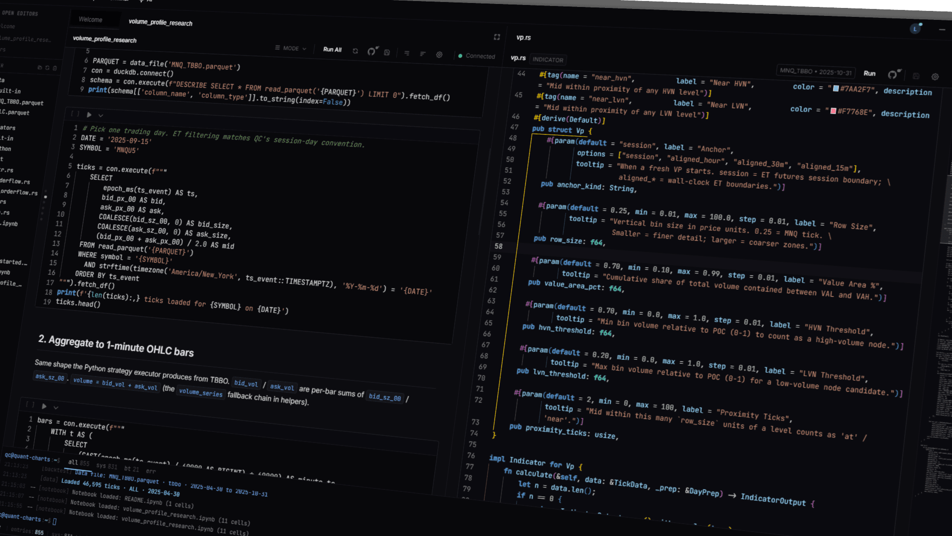
indicators/built-in/python/volume_profile.py
Programmable volume profile
Session VP with custom value-area math. Emits zone tags like bid_dom_at_poc and ask_dom_at_hvn for post-hoc filtering.
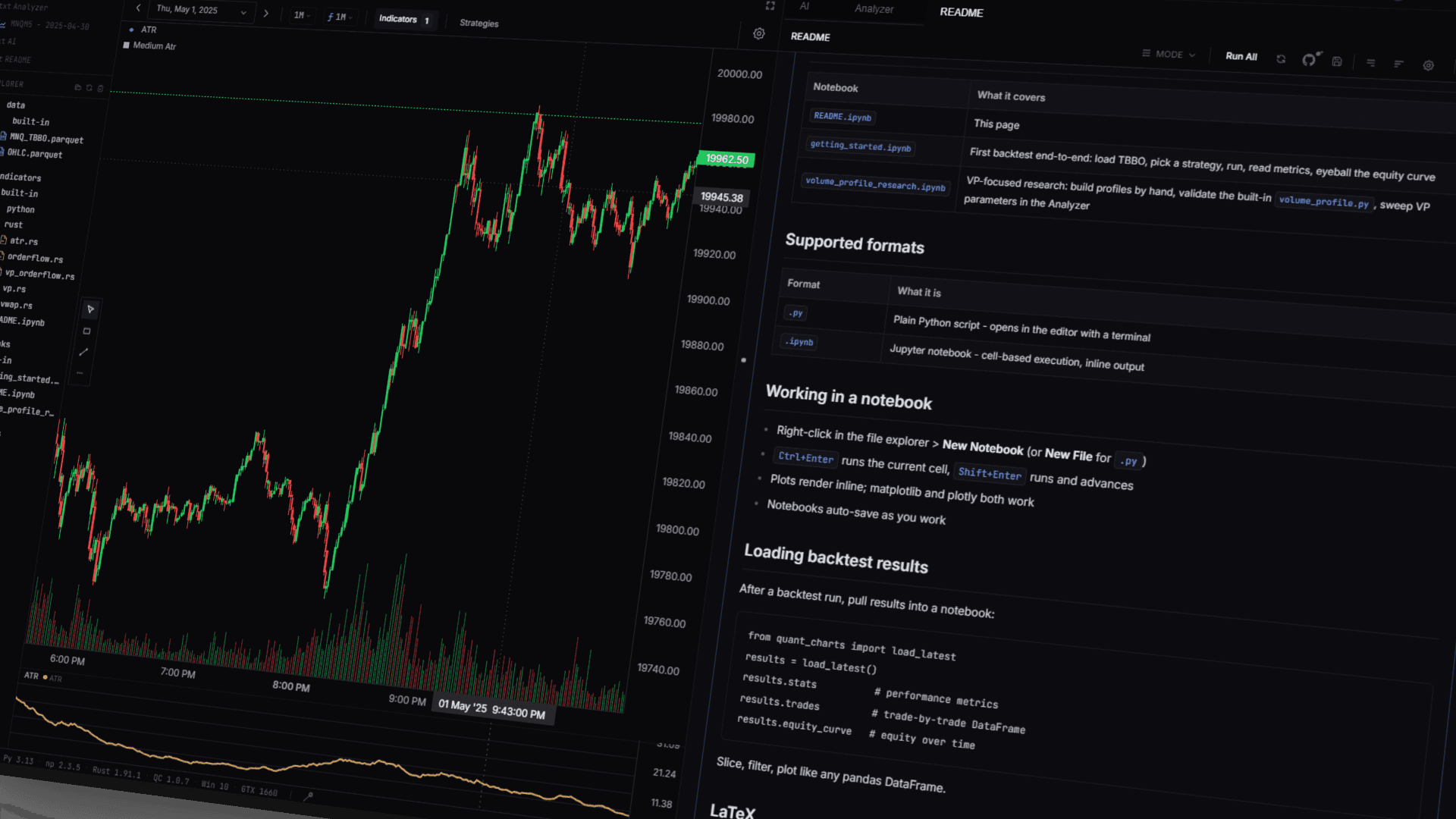
notebooks/built-in/getting_started.ipynb
Jupyter, in the workspace
Real Python kernel, not a sandbox. Pull the latest backtest result as a DataFrame; plot inline with matplotlib or plotly.
qc@quant-charts:~$
A terminal-grade research desk. Your code, your data, your machine.
Your code, on your disk
Quant Charts is a Python library and a Rust engine, running on your local disk. There is a custom API (the quant_charts package, the @strategy decorator, the engine it wires into), but the things you keep stay in formats you would keep anyway.
strategies
.py and .rs text files
Git versions them like any other source.
data
Apache Parquet
DuckDB, pandas, polars, Arrow, Spark all read it.
script_language
None. It is Python.
No Pine, no EasyLanguage, no NinjaScript.
if_we_shut_down
Files still open.
Rewrite the wiring, keep the math.
Get Quant Charts
$29.99 a month. Windows desktop. Cancel anytime. Lemon Squeezy, LLC handles the transaction; the app talks to your local disk for everything else. Create an account, or read the pricing details.